Convolution arithmetic tutorial
Note
This tutorial is adapted from an existing convolution arithmetic guide 1, with an added emphasis on Theano’s interface.
Also, note that the signal processing community has a different nomenclature and a well established literature on the topic, but for this tutorial we will stick to the terms used in the machine learning community. For a signal processing point of view on the subject, see for instance Winograd, Shmuel. Arithmetic complexity of computations. Vol. 33. Siam, 1980.
About this tutorial
Learning to use convolutional neural networks (CNNs) for the first time is generally an intimidating experience. A convolutional layer’s output shape is affected by the shape of its input as well as the choice of kernel shape, zero padding and strides, and the relationship between these properties is not trivial to infer. This contrasts with fully-connected layers, whose output size is independent of the input size. Additionally, so-called transposed convolutional layers (also known as fractionally strided convolutional layers, or – wrongly – as deconvolutions) have been employed in more and more work as of late, and their relationship with convolutional layers has been explained with various degrees of clarity.
The relationship between a convolution operation’s input shape, kernel size, stride, padding and its output shape can be confusing at times.
The tutorial’s objective is threefold:
Explain the relationship between convolutional layers and transposed convolutional layers.
Provide an intuitive understanding of the relationship between input shape, kernel shape, zero padding, strides and output shape in convolutional and transposed convolutional layers.
Clarify Theano’s API on convolutions.
Refresher: discrete convolutions
The bread and butter of neural networks is affine transformations: a vector is received as input and is multiplied with a matrix to produce an output (to which a bias vector is usually added before passing the result through a nonlinearity). This is applicable to any type of input, be it an image, a sound clip or an unordered collection of features: whatever their dimensionality, their representation can always be flattened into a vector before the transformation.
Images, sound clips and many other similar kinds of data have an intrinsic structure. More formally, they share these important properties:
They are stored as multi-dimensional arrays.
They feature one or more axes for which ordering matters (e.g., width and height axes for an image, time axis for a sound clip).
One axis, called the channel axis, is used to access different views of the data (e.g., the red, green and blue channels of a color image, or the left and right channels of a stereo audio track).
These properties are not exploited when an affine transformation is applied; in fact, all the axes are treated in the same way and the topological information is not taken into account. Still, taking advantage of the implicit structure of the data may prove very handy in solving some tasks, like computer vision and speech recognition, and in these cases it would be best to preserve it. This is where discrete convolutions come into play.
A discrete convolution is a linear transformation that preserves this notion of ordering. It is sparse (only a few input units contribute to a given output unit) and reuses parameters (the same weights are applied to multiple locations in the input).
Here is an example of a discrete convolution:
The light blue grid is called the input feature map. A kernel (shaded area) of value

slides across the input feature map. At each location, the product between each element of the kernel and the input element it overlaps is computed and the results are summed up to obtain the output in the current location. The final output of this procedure is a matrix called output feature map (in green).
This procedure can be repeated using different kernels to form as many output feature maps (a.k.a. output channels) as desired. Note also that to keep the drawing simple a single input feature map is being represented, but it is not uncommon to have multiple feature maps stacked one onto another (an example of this is what was referred to earlier as channels for images and sound clips).
Note
While there is a distinction between convolution and cross-correlation from a signal processing perspective, the two become interchangeable when the kernel is learned. For the sake of simplicity and to stay consistent with most of the machine learning literature, the term convolution will be used in this tutorial.
If there are multiple input and output feature maps, the collection of kernels
form a 4D array (output_channels, input_channels, filter_rows,
filter_columns). For each output channel, each input channel is convolved with
a distinct part of the kernel and the resulting set of feature maps is summed
elementwise to produce the corresponding output feature map. The result of this
procedure is a set of output feature maps, one for each output channel, that is
the output of the convolution.
The convolution depicted above is an instance of a 2-D convolution, but can be generalized to N-D convolutions. For instance, in a 3-D convolution, the kernel would be a cuboid and would slide across the height, width and depth of the input feature map.
The collection of kernels defining a discrete convolution has a shape
corresponding to some permutation of  , where
The following properties affect the output size  of a convolutional
layer along axis
of a convolutional
layer along axis  :
:
 : input size along axis ,
 : kernel size along axis ,
 : stride (distance between two consecutive positions of the
kernel) along axis ,
: stride (distance between two consecutive positions of the
kernel) along axis , : zero padding (number of zeros concatenated at the beginning and
at the end of an axis) along axis j.
: zero padding (number of zeros concatenated at the beginning and
at the end of an axis) along axis j.
For instance, here is a  kernel applied to a
 input padded with a
  border of zeros using
 strides:
The analysis of the relationship between convolutional layer properties is eased
by the fact that they don’t interact across axes, i.e., the choice of kernel
size, stride and zero padding along axis only affects the output size
of axis . Because of that, this section will focus on the following
simplified setting:
2-D discrete convolutions (
 ),
),square inputs (
 ),
),square kernel size (
 ),
),same strides along both axes (
 ),
),same zero padding along both axes (
 ).
).
This facilitates the analysis and the visualization, but keep in mind that the results outlined here also generalize to the N-D and non-square cases.
Theano terminology
Theano has its own terminology, which differs slightly from the convolution arithmetic guide’s. Here’s a simple conversion table for the two:
Theano |
Convolution arithmetic |
|---|---|
|
4D collection of kernels |
|
(batch size ( |
|
(output channels ( |
|
|
|
( |
 ,
,  )
)For instance, the convolution shown above would correspond to the following Theano call:
output = theano.tensor.nnet.conv2d(
    input, filters, input_shape=(1, 1, 5, 5), filter_shape=(1, 1, 3, 3),
    border_mode=(1, 1), subsample=(2, 2))
Convolution arithmetic
No zero padding, unit strides
The simplest case to analyze is when the kernel just slides across every
position of the input (i.e.,  and
and  ).
Here is an example for
).
Here is an example for  and
and  :
:
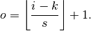
One way of defining the output size in this case is by the number of possible placements of the kernel on the input. Let’s consider the width axis: the kernel starts on the leftmost part of the input feature map and slides by steps of one until it touches the right side of the input. The size of the output will be equal to the number of steps made, plus one, accounting for the initial position of the kernel. The same logic applies for the height axis.
More formally, the following relationship can be inferred:
Relationship 1
For any  and
and  , and for and ,
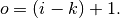
This translates to the following Theano code:
output = theano.tensor.nnet.conv2d(
    input, filters, input_shape=(b, c2, i1, i2), filter_shape=(c1, c2, k1, k2),
    border_mode=(0, 0), subsample=(1, 1))
# output.shape[2] == (i1 - k1) + 1
# output.shape[3] == (i2 - k2) + 1
Zero padding, unit strides
To factor in zero padding (i.e., only restricting to ), let’s
consider its effect on the effective input size: padding with  zeros
changes the effective input size from to
zeros
changes the effective input size from to  . In the
general case, Relationship 1 can then be used to infer the following
relationship:
. In the
general case, Relationship 1 can then be used to infer the following
relationship:
Relationship 2
For any , and , and for ,
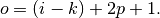
This translates to the following Theano code:
output = theano.tensor.nnet.conv2d(
    input, filters, input_shape=(b, c2, i1, i2), filter_shape=(c1, c2, k1, k2),
    border_mode=(p1, p2), subsample=(1, 1))
# output.shape[2] == (i1 - k1) + 2 * p1 + 1
# output.shape[3] == (i2 - k2) + 2 * p2 + 1
Here is an example for  ,
,  and
and  :
:
Special cases
In practice, two specific instances of zero padding are used quite extensively because of their respective properties. Let’s discuss them in more detail.
Half (same) padding
Having the output size be the same as the input size (i.e.,  ) can
be a desirable property:
) can
be a desirable property:
Relationship 3
For any and for odd ( ), and
  ,
,
This translates to the following Theano code:
output = theano.tensor.nnet.conv2d(
    input, filters, input_shape=(b, c2, i1, i2), filter_shape=(c1, c2, k1, k2),
    border_mode='half', subsample=(1, 1))
# output.shape[2] == i1
# output.shape[3] == i2
This is sometimes referred to as half (or same) padding. Here is an example
for , and (therefore)  :
:

Note that half padding also works for even-valued and for  , but in that case the property that the output size is the same as the input
size is lost. Some frameworks also implement the
, but in that case the property that the output size is the same as the input
size is lost. Some frameworks also implement the same convolution slightly
differently (e.g., in Keras 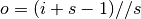 ).
).
Full padding
While convolving a kernel generally decreases the output size with respect to the input size, sometimes the opposite is required. This can be achieved with proper zero padding:
Relationship 4
For any and , and for  and
,
and
,
This translates to the following Theano code:
output = theano.tensor.nnet.conv2d(
    input, filters, input_shape=(b, c2, i1, i2), filter_shape=(c1, c2, k1, k2),
    border_mode='full', subsample=(1, 1))
# output.shape[2] == i1 + (k1 - 1)
# output.shape[3] == i2 + (k2 - 1)
This is sometimes referred to as full padding, because in this setting every
possible partial or complete superimposition of the kernel on the input feature
map is taken into account. Here is an example for ,
and (therefore) :
No zero padding, non-unit strides
All relationships derived so far only apply for unit-strided convolutions.
Incorporating non unitary strides requires another inference leap. To facilitate
the analysis, let’s momentarily ignore zero padding (i.e.,  and
). Here is an example for , and
and
). Here is an example for , and  :
:
Once again, the output size can be defined in terms of the number of possible
placements of the kernel on the input. Let’s consider the width axis: the kernel
starts as usual on the leftmost part of the input, but this time it slides by
steps of size  until it touches the right side of the input. The size
of the output is again equal to the number of steps made, plus one, accounting
for the initial position of the kernel. The same logic applies for the height
axis.
until it touches the right side of the input. The size
of the output is again equal to the number of steps made, plus one, accounting
for the initial position of the kernel. The same logic applies for the height
axis.
From this, the following relationship can be inferred:
Relationship 5
For any , and , and for ,
This translates to the following Theano code:
output = theano.tensor.nnet.conv2d(
    input, filters, input_shape=(b, c2, i1, i2), filter_shape=(c1, c2, k1, k2),
    border_mode=(0, 0), subsample=(s1, s2))
# output.shape[2] == (i1 - k1) // s1 + 1
# output.shape[3] == (i2 - k2) // s2 + 1
The floor function accounts for the fact that sometimes the last possible step does not coincide with the kernel reaching the end of the input, i.e., some input units are left out.
Zero padding, non-unit strides
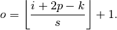
The most general case (convolving over a zero padded input using non-unit
strides) can be derived by applying Relationship 5 on an effective input of size
, in analogy to what was done for Relationship 2:
Relationship 6
For any , , and ,
This translates to the following Theano code:
output = theano.tensor.nnet.conv2d(
    input, filters, input_shape=(b, c2, i1, i2), filter_shape=(c1, c2, k1, k2),
    border_mode=(p1, p2), subsample=(s1, s2))
# output.shape[2] == (i1 - k1 + 2 * p1) // s1 + 1
# output.shape[3] == (i2 - k2 + 2 * p2) // s2 + 1
As before, the floor function means that in some cases a convolution will
produce the same output size for multiple input sizes. More specifically, if
 is a multiple of , then any input size
  will produce the same output size. Note
that this ambiguity applies only for .
will produce the same output size. Note
that this ambiguity applies only for .
Here is an example for , ,  and
and  :
:
Here is an example for  , , and :
Interestingly, despite having different input sizes these convolutions share the same output size. While this doesn’t affect the analysis for convolutions, this will complicate the analysis in the case of transposed convolutions.
Transposed convolution arithmetic
The need for transposed convolutions generally arises from the desire to use a transformation going in the opposite direction of a normal convolution, i.e., from something that has the shape of the output of some convolution to something that has the shape of its input while maintaining a connectivity pattern that is compatible with said convolution. For instance, one might use such a transformation as the decoding layer of a convolutional autoencoder or to project feature maps to a higher-dimensional space.
Once again, the convolutional case is considerably more complex than the fully-connected case, which only requires to use a weight matrix whose shape has been transposed. However, since every convolution boils down to an efficient implementation of a matrix operation, the insights gained from the fully-connected case are useful in solving the convolutional case.
Like for convolution arithmetic, the dissertation about transposed convolution arithmetic is simplified by the fact that transposed convolution properties don’t interact across axes.
This section will focus on the following setting:
2-D transposed convolutions (
),square inputs (
),square kernel size (
),same strides along both axes (
),same zero padding along both axes (
).
Once again, the results outlined generalize to the N-D and non-square cases.
Convolution as a matrix operation
Take for example the convolution presented in the No zero padding, unit strides subsection:
If the input and output were to be unrolled into vectors from left to right, top
to bottom, the convolution could be represented as a sparse matrix
 where the non-zero elements are the elements
  of the kernel (with and being the row and column of the
kernel respectively):
of the kernel (with and being the row and column of the
kernel respectively):
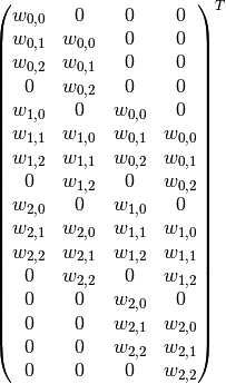
(Note: the matrix has been transposed for formatting purposes.) This linear
operation takes the input matrix flattened as a 16-dimensional vector and
produces a 4-dimensional vector that is later reshaped as the
output matrix.
Using this representation, the backward pass is easily obtained by transposing
; in other words, the error is backpropagated by multiplying
the loss with  . This operation takes a 4-dimensional vector
as input and produces a 16-dimensional vector as output, and its connectivity
pattern is compatible with by construction.
. This operation takes a 4-dimensional vector
as input and produces a 16-dimensional vector as output, and its connectivity
pattern is compatible with by construction.
Notably, the kernel  defines both the matrices
and used for the forward and backward
passes.
defines both the matrices
and used for the forward and backward
passes.
Transposed convolution
Let’s now consider what would be required to go the other way around, i.e., map from a 4-dimensional space to a 16-dimensional space, while keeping the connectivity pattern of the convolution depicted above. This operation is known as a transposed convolution.
Transposed convolutions – also called fractionally strided convolutions – work by swapping the forward and backward passes of a convolution. One way to put it is to note that the kernel defines a convolution, but whether it’s a direct convolution or a transposed convolution is determined by how the forward and backward passes are computed.
For instance, the kernel defines a convolution whose forward
and backward passes are computed by multiplying with and
respectively, but it also defines a transposed
convolution whose forward and backward passes are computed by multiplying with
and  respectively.
Note
The transposed convolution operation can be thought of as the gradient of some convolution with respect to its input, which is usually how transposed convolutions are implemented in practice.
Finally note that it is always possible to implement a transposed convolution with a direct convolution. The disadvantage is that it usually involves adding many columns and rows of zeros to the input, resulting in a much less efficient implementation.
Building on what has been introduced so far, this section will proceed somewhat backwards with respect to the convolution arithmetic section, deriving the properties of each transposed convolution by referring to the direct convolution with which it shares the kernel, and defining the equivalent direct convolution.
No zero padding, unit strides, transposed
The simplest way to think about a transposed convolution is by computing the output shape of the direct convolution for a given input shape first, and then inverting the input and output shapes for the transposed convolution.
Let’s consider the convolution of a kernel on a  input with unitary stride and no padding (i.e., ,
, and ). As depicted in the convolution
below, this produces a output:
input with unitary stride and no padding (i.e., ,
, and ). As depicted in the convolution
below, this produces a output:
The transpose of this convolution will then have an output of shape when applied on a input.
Another way to obtain the result of a transposed convolution is to apply an
equivalent – but much less efficient – direct convolution. The example
described so far could be tackled by convolving a kernel over
a input padded with a border of zeros
using unit strides (i.e.,  ,
,  ,
,  and
and
 ), as shown here:
Notably, the kernel’s and stride’s sizes remain the same, but the input of the equivalent (direct) convolution is now zero padded.
Note
Although equivalent to applying the transposed matrix, this visualization adds a lot of zero multiplications in the form of zero padding. This is done here for illustration purposes, but it is inefficient, and software implementations will normally not perform the useless zero multiplications.
One way to understand the logic behind zero padding is to consider the connectivity pattern of the transposed convolution and use it to guide the design of the equivalent convolution. For example, the top left pixel of the input of the direct convolution only contribute to the top left pixel of the output, the top right pixel is only connected to the top right output pixel, and so on.
To maintain the same connectivity pattern in the equivalent convolution it is necessary to zero pad the input in such a way that the first (top-left) application of the kernel only touches the top-left pixel, i.e., the padding has to be equal to the size of the kernel minus one.
Proceeding in the same fashion it is possible to determine similar observations for the other elements of the image, giving rise to the following relationship:
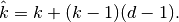
Relationship 7
A convolution described by , and has an
associated transposed convolution described by ,  and
and  and its output size is
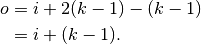
In other words,
input = theano.tensor.nnet.abstract_conv.conv2d_grad_wrt_inputs(
    output, filters, filter_shape=(c1, c2, k1, k2), border_mode=(0, 0),
    subsample=(1, 1))
# input.shape[2] == output.shape[2] + (k1 - 1)
# input.shape[3] == output.shape[3] + (k2 - 1)
Interestingly, this corresponds to a fully padded convolution with unit strides.
Zero padding, unit strides, transposed
Knowing that the transpose of a non-padded convolution is equivalent to convolving a zero padded input, it would be reasonable to suppose that the transpose of a zero padded convolution is equivalent to convolving an input padded with less zeros.
It is indeed the case, as shown in here for , and
:
Formally, the following relationship applies for zero padded convolutions:
Relationship 8
A convolution described by , and has an
associated transposed convolution described by , and  and its output size is
In other words,
input = theano.tensor.nnet.abstract_conv.conv2d_grad_wrt_inputs(
    output, filters, filter_shape=(c1, c2, k1, k2), border_mode=(p1, p2),
    subsample=(1, 1))
# input.shape[2] == output.shape[2] + (k1 - 1) - 2 * p1
# input.shape[3] == output.shape[3] + (k2 - 1) - 2 * p2
Special cases
Half (same) padding, transposed
By applying the same inductive reasoning as before, it is reasonable to expect that the equivalent convolution of the transpose of a half padded convolution is itself a half padded convolution, given that the output size of a half padded convolution is the same as its input size. Thus the following relation applies:
Relationship 9
A convolution described by  ,
and has an associated
transposed convolution described by ,
,
and has an associated
transposed convolution described by ,  and
and
 and its output size is
In other words,
input = theano.tensor.nnet.abstract_conv.conv2d_grad_wrt_inputs(
    output, filters, filter_shape=(c1, c2, k1, k2), border_mode='half',
    subsample=(1, 1))
# input.shape[2] == output.shape[2]
# input.shape[3] == output.shape[3]
Here is an example for , and (therefore)  :
:
Full padding, transposed
Knowing that the equivalent convolution of the transpose of a non-padded convolution involves full padding, it is unsurprising that the equivalent of the transpose of a fully padded convolution is a non-padded convolution:
Relationship 10
A convolution described by , and
has an associated transposed convolution described by ,
and  and its output size is
In other words,
input = theano.tensor.nnet.abstract_conv.conv2d_grad_wrt_inputs(
    output, filters, filter_shape=(c1, c2, k1, k2), border_mode='full',
    subsample=(1, 1))
# input.shape[2] == output.shape[2] - (k1 - 1)
# input.shape[3] == output.shape[3] - (k2 - 1)
Here is an example for , and (therefore)  :
:
No zero padding, non-unit strides, transposed
Using the same kind of inductive logic as for zero padded convolutions, one
might expect that the transpose of a convolution with involves an
equivalent convolution with  . As will be explained, this is a valid
intuition, which is why transposed convolutions are sometimes called
fractionally strided convolutions.
. As will be explained, this is a valid
intuition, which is why transposed convolutions are sometimes called
fractionally strided convolutions.
Here is an example for , and :
This should help understand what fractional strides involve: zeros are inserted between input units, which makes the kernel move around at a slower pace than with unit strides.
Note
Doing so is inefficient and real-world implementations avoid useless multiplications by zero, but conceptually it is how the transpose of a strided convolution can be thought of.
For the moment, it will be assumed that the convolution is non-padded ( ) and that its input size is such that
  is a multiple
of . In that case, the following relationship holds:
is a multiple
of . In that case, the following relationship holds:
Relationship 11
A convolution described by , and and whose
input size is such that is a multiple of , has an
associated transposed convolution described by  ,
,  , and , where is the
size of the stretched input obtained by adding
, and , where is the
size of the stretched input obtained by adding  zeros between
each input unit, and its output size is
zeros between
each input unit, and its output size is
In other words,
input = theano.tensor.nnet.abstract_conv.conv2d_grad_wrt_inputs(
    output, filters, filter_shape=(c1, c2, k1, k2), border_mode=(0, 0),
    subsample=(s1, s2))
# input.shape[2] == s1 * (output.shape[2] - 1) + k1
# input.shape[3] == s2 * (output.shape[3] - 1) + k2
Zero padding, non-unit strides, transposed
When the convolution’s input size is such that is a
multiple of , the analysis can extended to the zero padded case by
combining Relationship 8 and
Relationship 11:
Relationship 12
A convolution described by , and and whose
input size is such that is a multiple of
has an associated transposed convolution described by
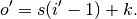
, , and 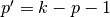 , where is the size of the stretched input obtained by
adding zeros between each input unit, and its output size is
, where is the size of the stretched input obtained by
adding zeros between each input unit, and its output size is
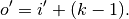
In other words,
o_prime1 = s1 * (output.shape[2] - 1) + k1 - 2 * p1
o_prime2 = s2 * (output.shape[3] - 1) + k2 - 2 * p2
input = theano.tensor.nnet.abstract_conv.conv2d_grad_wrt_inputs(
    output, filters, input_shape=(b, c1, o_prime1, o_prime2),
    filter_shape=(c1, c2, k1, k2), border_mode=(p1, p2),
    subsample=(s1, s2))
Here is an example for , , and :
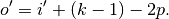
The constraint on the size of the input can be relaxed by introducing
another parameter  that allows to distinguish
between the different cases that all lead to the same
that allows to distinguish
between the different cases that all lead to the same  :
:
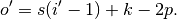
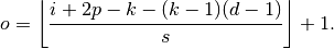
Relationship 13
A convolution described by , and has an
associated transposed convolution described by  ,
, , and , where is the size of the stretched input obtained by
adding zeros between each input unit, and
,
, , and , where is the size of the stretched input obtained by
adding zeros between each input unit, and  represents the number of zeros added to the top and right edges
of the input, and its output size is
represents the number of zeros added to the top and right edges
of the input, and its output size is

In other words,
o_prime1 = s1 * (output.shape[2] - 1) + a1 + k1 - 2 * p1
o_prime2 = s2 * (output.shape[3] - 1) + a2 + k2 - 2 * p2
input = theano.tensor.nnet.abstract_conv.conv2d_grad_wrt_inputs(
    output, filters, input_shape=(b, c1, o_prime1, o_prime2),
    filter_shape=(c1, c2, k1, k2), border_mode=(p1, p2),
    subsample=(s1, s2))
Here is an example for , , and :
Miscellaneous convolutions
Dilated convolutions
Those familiar with the deep learning literature may have noticed the term “dilated convolutions” (or “atrous convolutions”, from the French expression convolutions à trous) appear in recent papers. Here we attempt to provide an intuitive understanding of dilated convolutions. For a more in-depth description and to understand in what contexts they are applied, see Chen et al. (2014) 2; Yu and Koltun (2015) 3.
Dilated convolutions “inflate” the kernel by inserting spaces between the kernel
elements. The dilation “rate” is controlled by an additional hyperparameter
 . Implementations may vary, but there are usually
  spaces
inserted between kernel elements such that
spaces
inserted between kernel elements such that  corresponds to a
regular convolution.
corresponds to a
regular convolution.
To understand the relationship tying the dilation rate and the output
size  , it is useful to think of the impact of on the
effective kernel size. A kernel of size dilated by a factor
has an effective size
, it is useful to think of the impact of on the
effective kernel size. A kernel of size dilated by a factor
has an effective size
This can be combined with Relationship 6 to form the following relationship for dilated convolutions:
Relationship 14
For any , , and , and for a dilation
rate ,
This translates to the following Theano code using the filter_dilation
parameter:
output = theano.tensor.nnet.conv2d(
    input, filters, input_shape=(b, c2, i1, i2), filter_shape=(c1, c2, k1, k2),
    border_mode=(p1, p2), subsample=(s1, s2), filter_dilation=(d1, d2))
# output.shape[2] == (i1 + 2 * p1 - k1 - (k1 - 1) * (d1 - 1)) // s1 + 1
# output.shape[3] == (i2 + 2 * p2 - k2 - (k2 - 1) * (d2 - 1)) // s2 + 1
Here is an example for  , ,
, ,  ,
,  and :
and :
- 1
Dumoulin, Vincent, and Visin, Francesco. “A guide to convolution arithmetic for deep learning”. arXiv preprint arXiv:1603.07285 (2016)
- 2
Chen, Liang-Chieh, Papandreou, George, Kokkinos, Iasonas, Murphy, Kevin and Yuille, Alan L. “Semantic image segmentation with deep convolutional nets and fully connected CRFs”. arXiv preprint arXiv:1412.7062 (2014).
- 3
Yu, Fisher and Koltun, Vladlen. “Multi-scale context aggregation by dilated convolutions”. arXiv preprint arXiv:1511.07122 (2015)
Grouped Convolutions
In grouped convolutions with  number of groups, the input and kernel
are split by their channels to form distinct groups. Each group
performs convolutions independent of the other groups to give
different outputs. These individual outputs are then concatenated together to give
the final output. A few examples of works using grouped convolutions are Krizhevsky et al (2012) 4;
Xie et at (2016) 5.
number of groups, the input and kernel
are split by their channels to form distinct groups. Each group
performs convolutions independent of the other groups to give
different outputs. These individual outputs are then concatenated together to give
the final output. A few examples of works using grouped convolutions are Krizhevsky et al (2012) 4;
Xie et at (2016) 5.
A special case of grouped convolutions is when equals the number of input
channels. This is called depth-wise convolutions or channel-wise convolutions.
depth-wise convolutions also forms a part of separable convolutions.
An example to use Grouped convolutions would be:
output = theano.tensor.nnet.conv2d(
    input, filters, input_shape=(b, c2, i1, i2), filter_shape=(c1, c2 / n, k1, k2),
    border_mode=(p1, p2), subsample=(s1, s2), filter_dilation=(d1, d2), num_groups=n)
# output.shape[0] == b
# output.shape[1] == c1
# output.shape[2] == (i1 + 2 * p1 - k1 - (k1 - 1) * (d1 - 1)) // s1 + 1
# output.shape[3] == (i2 + 2 * p2 - k2 - (k2 - 1) * (d2 - 1)) // s2 + 1
- 4
Alex Krizhevsky, Ilya Sutskever, Geoffrey E. Hinton. “ImageNet Classification with Deep Convolutional Neural Networks”. Advances in Neural Information Processing Systems 25 (NIPS 2012)
- 5
Saining Xie, Ross Girshick, Piotr Dollár, Zhuowen Tu, Kaiming He. “Aggregated Residual Transformations for Deep Neural Networks”. arxiv preprint arXiv:1611.05431 (2016).
Separable Convolutions
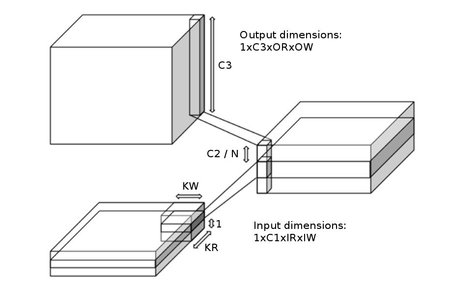
Separable convolutions consists of two consecutive convolution operations. First is depth-wise convolutions which performs convolutions separately for each channel of the input. The output of this operation is the given as input to point-wise convolutions which is a special case of general convolutions with 1x1 filters. This mixes the channels to give the final output.
As we can see from this diagram, modified from Vanhoucke(2014) 6, depth-wise
convolutions is performed with  single channel depth-wise filters
to give a total of output channels in the intermediate output where
each channel in the input separately performs convolutions with separate kernels
to give
single channel depth-wise filters
to give a total of output channels in the intermediate output where
each channel in the input separately performs convolutions with separate kernels
to give  channels to the intermediate output, where is
the number of input channels. The intermediate output then performs point-wise
convolutions with
channels to the intermediate output, where is
the number of input channels. The intermediate output then performs point-wise
convolutions with  1x1 filters which mixes the channels of the intermediate
output to give the final output.
1x1 filters which mixes the channels of the intermediate
output to give the final output.
Separable convolutions is used as follows:
output = theano.tensor.nnet.separable_conv2d(
    input, depthwise_filters, pointwise_filters, num_channels = c1,
    input_shape=(b, c1, i1, i2), depthwise_filter_shape=(c2, 1, k1, k2),
    pointwise_filter_shape=(c3, c2, 1, 1), border_mode=(p1, p2),
    subsample=(s1, s2), filter_dilation=(d1, d2))
# output.shape[0] == b
# output.shape[1] == c3
# output.shape[2] == (i1 + 2 * p1 - k1 - (k1 - 1) * (d1 - 1)) // s1 + 1
# output.shape[3] == (i2 + 2 * p2 - k2 - (k2 - 1) * (d2 - 1)) // s2 + 1
- 6
Vincent Vanhoucke. “Learning Visual Representations at Scale”, International Conference on Learning Representations(2014).
Quick reference
Convolution relationship
A convolution specified by
input size
,kernel size
,stride
,padding size
,
has an output size given by
In Theano, this translates to
output = theano.tensor.nnet.conv2d(
    input, filters, input_shape=(b, c2, i1, i2), filter_shape=(c1, c2, k1, k2),
    border_mode=(p1, p2), subsample=(s1, s2))
# output.shape[2] == (i1 + 2 * p1 - k1) // s1 + 1
# output.shape[3] == (i2 + 2 * p2 - k2) // s2 + 1
Transposed convolution relationship
A transposed convolution specified by
input size
,kernel size
,stride
,padding size
,
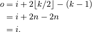
has an output size given by

where is a user-specified quantity used to distinguish between the
different possible output sizes.
Unless , Theano requires that is implicitly passed
via an input_shape argument. For instance, if  ,
, , and
,
, , and  , then
 and the Theano code would look like
input = theano.tensor.nnet.abstract_conv.conv2d_grad_wrt_inputs(
    output, filters, input_shape=(9, 9), filter_shape=(c1, c2, 4, 4),
    border_mode='valid', subsample=(2, 2))